Think about an image of a squirrel floating in space, like the one in the video above. How can a computer understand what the image represents? What if we could teach a machine to read an image more like how we read text, by looking at meaningful chunks and understanding their relationships? Introducing Vision Transformers. Transformers power all the latest advances in AI, from Gemini to ChatGPT, Claude, LLaMa, and pretty much every big model you’ve heard of in the last two years. They are known to be ground-breaking language models, but they are also extremely powerful at solving computer vision tasks.

In this post, we’ll understand what a Vision Transformer is and how it works in detail. We’ll build and train a Vision Transformer from scratch to classify images. I’ll focus on intuition, explaining the why behind each component, and walk through the code step-by-step. I have included some quizzes and recaps along the way to reinforce understanding - spaced repetition! 🙌 The code for this blog post is here

We’ll build and train using Google’s JAX and the new NNX library. NNX makes building complex models like ViTs more explicit and Pythonic. Why JAX/NNX? JAX is extremely efficient thanks to jit (just-in-time) compilation and fast automatic differentiation (grad). It also runs seamlessly on CPU/GPU/TPU. This great post covers its benefits: PyTorch is Dead. Long Live Jax (Disclaimer: I wouldn’t say PyTorch is dead, I love PyTorch. But JAX is equally cool!).NNX is the new deep learning framework for JAX, which is currently Google’s recommended framework and provides a more familiar object-oriented programming model (like PyTorch) while retaining JAX’s functional principles.

Important resources:

Original paper: An Image is Worth 16x16 Words, Dosovitskiy et al.
Code for this blog post

# Seeing the World Through Transformers

Remember our squirrel image? How can a Transformer, designed for text sequences, process it? The core idea is simple:

• Patchify: We first divide the image into smaller, fixed-size patches.
• Flatten & Embed: Each patch is just a collection of raw pixel data. To make sense of it, we need to convert each patch into a meaningful vector, or embedding. We flatten each patch and linearly project it into an embedding vector using a learnable transformation.
• Add Position Info: A Transformer doesn’t inherently know patch order. It processes all patches in parallel. We add positional embeddings to retain spatial information.
• CLS Token: We add a special classification token embedding at position 0 in the embedding sequence. This token will learn to aggregate global image information.
• Attention Magic: Each embedding “looks” at all the other embeddings and decides which ones are most important to understand its own context. This is done through multiple layers of self-attention.
• Classify: We use the output corresponding to the CLS token to predict the image’s class.

Overview of the main steps in a Vision Transformer. Source: original paper

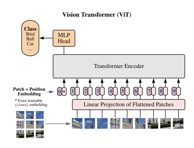
This is a high-level overview of the Vision Transformer architecture. Let’s build each part.

## Step 1: Patchifying the Image, From Pixels to Patches

First, we need to break the image down into patches. Think of this like cutting a photo into a grid of smaller squares. Instead of processing pixel by pixel like a Convolutional Neural Network does, we treat chunks of the image as the fundamental units. This mimicks what happens in a sentence, where the fundamental input units are individual words (technically, chunks of words or tokens). Slicing the image into tiny patches allows the Transformer to later find relationships between different parts of the image.

We use the einops library for elegant tensor manipulation. einops is beautiful, but can be cryptic. Here’s what we do below in the patchify_image() function:

• We want to rearrange the pattern from (Batch, Height, Width, Channels) to (Batch, Num_Patches, Patch_Dimension).
• "... (h p1) (w p2) c -> ... (h w) (p1 p2 c)":
  • (h p1): The Height dimension is composed of h patches, each of height p1 (patch_size).
  • (w p2): The Width dimension is composed of w patches, each of width p2 (patch_size).
  • c: The Channels dimension (in our case c=3 for an RGB image).
• -> ... (h w): The output sequence length is h * w (total number of patches, N).
• (p1 p2 c): Each element in the sequence is a flattened patch of size p1 * p2 * c (the patch dimension, D_patch).

    # From src/transformer.py
    import einops
    import jax.numpy as jnp
    import functools
    from flax import nnx
    import jaxtyping as jt
    
    Float = jt.Float
    Array = jt.Array
    
    @functools.partial(jax.jit, static_argnames=("patch_size",))
    def patchify_image(
        image: Float[Array, "B H W C"], patch_size: int
    ) -> Float[Array, "B N D_patch"]: # N = (H/patch_size)*(W/patch_size), D_patch = patch_size*patch_size*C
        # Rearranges image from (Batch, Height, Width, Channels)
        # to (Batch, Num_Patches, Patch_Height * Patch_Width * Channels)
        patches = einops.rearrange(
            image,
            "... (h p1) (w p2) c -> ... (h w) (p1 p2 c)", # h, w are counts of patches
            p1=patch_size, # p1 = patch height
            p2=patch_size, # p2 = patch width
        )
        return patches
    

This function takes a batch of images (B, H, W, C) and reshapes it into a batch of sequences of flattened patches (B, NumPatches, PatchSize*PatchSize*C).

Assuming:

• input image is (1, 224, 224, 3) and patch_size is 16
• then h = 224/16 = 14, w = 224/16 = 14.
• Number of patches N = h * w = 14 * 14 = 196.
• Patch dimension D_patch = p1 * p2 * c = 16 * 16 * 3 = 768.
• The output shape would be (1, 196, 768).

The decorator @functools.partial(jax.jit, static_argnames=("patch_size",)) applied to the function makes sure that JAX compiles this function for massive speedups on GPUs/TPUs. The argument static_argnames=("patch_size",) tells the JAX compiler that patch_size is static: its value is known at compile time and won’t change during execution for that compiled version. JAX needs this information because patch_size is a Python integer, not a JAX tensor, and its value affects the tensor shapes, which must be static for compilation.

## Step 2: Patch Embedding

Raw pixel patches aren’t ideal for a Transformer. Pixel colors are simply intensity values, telling us the contribution of the Red, Green, and Blue channels. Pixels do not inherently encode semantic information, and they are very sensitive to noise and minor shifts in lighting. We need to map these raw patches to more useful, richer representations. The goal is to train our model to extract features that are relevant for the task at hand (e.g. image classification). In other words, we need to project raw pixel patches into a learned embedding space, similarly to how words are embedded into high dimensional vectors in Natural Language Processing.

We use a standard Linear layer (nnx.Linear), a simple matrix multiplication + bias, to transform each flattened patch (e.g., 768 dimensions if patch size is 16x16 and 3 channels) into a desired embedding dimension (dim_emb, often 768 or higher in larger models). This layer’s weights are learned during training, allowing it to discover how to best extract useful features from the raw patches. We define an nnx.Module for this. NNX encourages organizing parameters and logic together within modules following an object-oriented style. We define a PatchEmbedding class inheriting from nnx.Module. Notice that nnx.Linear requires rngs (random number generators). This is a key aspect of JAX/NNX: randomness (for weight initialization) must be explicitly handled via Random Number Generator keys (jax.random.PRNGKey) to ensures reproducibility. nnx.Rngs is a helper to manage these keys.

# From src/transformer.py
class PatchEmbedding(nnx.Module):
    """Patch embedding module."""
    def __init__(self, patch_size: int, out_features: int, rngs: nnx.Rngs):
        self.patch_size = patch_size
        self.out_features = out_features 
        self.channels = 3 # Assuming RGB images
        # A linear layer to project flattened patches
        self.linear = nnx.Linear(
            in_features=self.patch_size**2 * self.channels, # e.g., 16*16*3 = 768
            out_features=self.out_features, # e.g. 768
            rngs=rngs # NNX requires explicit RNG handling
        )

    def __call__(self, inputs: Float[Array, "B H W C"]) -> Float[Array, "B N D_emb"]:
        # Patchify the image using the function from Step 1
        patches = patchify_image(inputs, self.patch_size) # (B, N, P*P*C)
        # Apply the learned linear projection
        projection = self.linear(patches) # (B, N, D_emb)
        return projection
    

This module takes the raw image, patchifies it internally using our previous patchify_image function, and then passes the sequence of flattened patches through a nnx.Linear layer to get the final patch embeddings. Each patch is now represented by a vector of out_features dimensions.

## Step 3: Positional Embeddings

Standard Transformers are permutation-invariant, which means they treat input elements as an unordered set, not a sequence. In other words, they process patches in parallel, without any information on where each patch came from in the original image. But for images, the location of a patch matters! Sky above a tree depicts a landscape, while sky below a tree might suggest a lake and its reflection. We need to give the model information about each patch’s original location. Instead of simply feeding in the raw index of a patch (like patch #1, #2, etc.), we use positional embeddings. These are learned vectors, one for each possible patch position in the sequence. Think of them as encoding the “address” or “coordinates” of each patch into a vector, allowing the model to understand the image’s structure. The vector has the same dimensionality of the patch embeddings, so they can be directly added together.

Why don’t we simply use the raw index? While fixed positional encodings (like sine/cosine functions) are an option, using learnable embeddings (nnx.Param) gives the model maximum flexibility. The model can learn the optimal way to represent position for the specific task and dataset. These learned embeddings can capture more complex spatial relationships than fixed schemes: for example, patches that are close together might have more similar embeddings.

# From src/transformer.py
class PositionalEmbedding(nnx.Module):
    def __init__(self, in_features: int, out_features: int, rngs: nnx.Rngs):
        """Initialize the Positional Embedding module.
        
        Args:
            in_features: The input dimension, typically number of patches + 1 (for CLS token).
            out_features: The output embedding dimension (dim_emb).
            rngs: The random number generator state.
        """
        self.in_features = in_features # Sequence length (NumPatches + 1 for CLS)
        self.out_features = out_features # Embedding dimension (dim_emb)
        key = rngs.params() # Get a JAX PRNGKey for initialization

    def __call__(self) -> Float[Array, "1 M D_emb"]: # M = NumPatches + 1
        # Simply returns the learned embedding table
        return self.pos_embedding
    

We create a learnable nnx.Param tensor called pos_embedding. Its shape is (1, NumPatches + 1, EmbeddingDim). We initialize these embeddings with small random values (scaled by 0.02). The + 1 in NumPatches + 1 is for the special [CLS] classification token, which we’ll introduce next.

## Step 4: The CLS Token

Inspired by BERT, ViTs add an extra learnable embedding to the sequence of patch embeddings, usually at the beginning (position 0). This is called the [CLS] (classification) token. Think of this token as a special “summary” embedding. This token has no direct input from the image pixels; it starts as a learned placeholder. The idea is that through the self-attention mechanism (coming next in Step 5!), will interact with all the patch embeddings. As information flows through the Transformer layers, the CLS token acts like a ‘sponge’, aggregating global information from the entire sequence of patch embeddings. At the end of the Transformer, we can just use the output embedding corresponding to this CLS token to make the final image classification decision. This simplifies the architecture by providing a single, aggregated vector representation of the image ready for the classification head, rather than, say, averaging all patch embeddings.

# From src/transformer.py
# Inside VisionTransformer.__init__
self.cls_embedding = nnx.Param(
    # A single learnable embedding vector of dimension dim_emb
    jax.random.normal(key=self.rngs.params(), shape=(1, self.dim_emb)) * 0.02
)

# Function to prepend the CLS token
def add_classification_token(
    cls_embedding: Float[Array, "1 D_emb"],
    embeddings: Float[Array, "B N D_emb"]
) -> Float[Array, "B M D_emb"]: # M = N + 1 (Sequence length becomes NumPatches + 1)
    # Repeat CLS token for each item in the batch
    cls_embedding_batch = jnp.tile(
        cls_embedding, (embeddings.shape[0], 1, 1) # Shape becomes (B, 1, D_emb)
    )
    # Concatenate CLS token at the beginning of the patch sequence (axis 1 is sequence dimension)
    return jnp.concatenate([cls_embedding_batch, embeddings], axis=1)
    

In the VisionTransformer class we define cls_embedding as another learnable nnx.Param. The add_classification_token() function takes this single CLS token, expands it to match the batch size of the patch embeddings using jnp.tile, and then prepends it to the sequence of patch embeddings. The positional embeddings are then added to this combined sequence.

Now we have a sequence of embeddings ready for the Transformer Encoder! The shape of this sequence is (Batch, NumPatches + 1, EmbeddingDim).

## Step 5: Attention and the Transformer Encoder

Attention: this is the heart of the ViT. Let’s start with building a strong intuition for the self-attention mechanism. Imagine each token in our sequence (patch embeddings + CLS token) wants to update itself by gathering information from other tokens. To do this, each token generates three vectors from its own embedding: a Query (Q) representing its current state and what it’s looking for, a Key (K) representing what it can offer, and a Value (V) representing the actual content it wants to share. These Q, K, V vectors are typically derived by multiplying the token’s embedding by three separate learnable weight matrices (W_Q, W_K, W_V).

The attention procedures compares its Query with the Keys of all other tokens (including itself). High similarity (dot product) means high relevance. These similarities become attention scores, which are normalized via softmax. The Query token then takes a weighted sum of all tokens’ Values, using these attention weights. It pays more attention to tokens relevant to its Query. in other words, this process allows each token (patch embedding or CLS token) to “look” at all other tokens in the sequence and decide which ones are most relevant to it. It calculates attention scores, determining how much “focus” to place on other tokens when updating its own representation.

In practice, we usually don’t use a single set of W_Q, W_K, W_V matrices. We use multiple sets in parallel, and this is called Multi-Head Self Attention. Each head performs the attention mechanism independently with its own learned projection matrices. This allows the model to capture different types of relationships and focus on different aspects of the information (e.g. one head might focus on texture, another on shapes, another on long-range dependencies). The outputs of these heads are then concatenated and linearly projected back to the original embedding dimension.

The attention magic happens in the Transformer Encoder, which is typically a stack of identical Encoder Blocks. Each block processes the sequence of embeddings, allowing tokens to interact and exchange information.

Encoder Block. Source

An Encoder Block usually contains:

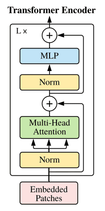
• Layer Normalization
• Multi-Head Self-Attention (MHSA)
• Skip Connection (Residual)
• Layer Normalization
• Feed-Forward Network (MLP)
• Skip Connection (Residual)

Dropout is also typically applied for regularization.

Let’s look at the code for these components:

Layer Normalization (LayerNorm): This normalizes the activations across the embedding dimension for each token independently. It helps stabilize training and improve generalization by ensuring that the inputs to subsequent layers are within a consistent range. Our LayerNorm is parameter-free. This is not common, but I read this paper showing that parameters in this layer might not be always beneficial for training.

# From src/transformer.py
class LayerNorm(nnx.Module):
    """Layer normalization module."""
    def __call__(self, x: Float[Array, "B N D"]) -> Float[Array, "B N D"]:
        x_mean = jnp.mean(x, axis=-1, keepdims=True)
        x_std = jnp.std(x, axis=-1, keepdims=True)
        return (x - x_mean) / (x_std + 1e-6) # Add epsilon for numerical stability
    

Multi-Head Attention (MultiHeadAttention): This module implements the core attention logic. Before looking at the code, it’s important to understand what the key steps are:

1. Input x (shape B, N, D_emb) is linearly projected into Q, K, V (each of shape B, N, D_qkv).
2. Q, K, V are reshaped and transposed by split_attention_heads to (B, num_heads, N, D_head_qkv).
3. Scaled dot-product attention scores are computed: scores = (Q_h @ K_h^T) / sqrt(D_head_qkv). The scaling by sqrt(D_head_qkv) prevents very large values when D_head_qkv is large, which could push softmax into regions with tiny gradients.
4. softmax is applied to scores to get attention weights.
5. Weights are multiplied by V_h to get the output for each head.
6. Outputs from all heads are concatenated and passed through a final linear layer (self.out).
7. Dropout is applied for regularization.

Please note that the code on GitHub evolves and might have slightly different wording and fewer comments. In this blog post I’m optimizing for clarity, while the code on GitHub is a bit more concise. However the mechanism is exactly the same.

# From src/transformer.py
def split_attention_heads(x, num_heads, dim_head):
    # (B, N, D_qkv) -> (B, N, num_heads, D_head)
    batch_size, num_patches = x.shape[:2]
    x = x.reshape((batch_size, num_patches, num_heads, dim_head))
    # (B, N, num_heads, D_head) -> (B, num_heads, N, D_head)
    x = jnp.transpose(x, (0, 2, 1, 3))
    return x

class MultiHeadAttention(nnx.Module):
    """Multi-head attention module."""
    def __init__(self, num_heads: int, dim_qkv: int, dim_emb: int, dim_out: int, rngs: nnx.Rngs):
        self.num_heads = num_heads
        self.dim_qkv = dim_qkv # Total dimension for Q, K, V across all heads
        self.dim_emb = dim_emb # Input embedding dimension
        self.dim_out = dim_out # Output dimension

        self.head_dim_qkv = self.dim_qkv // self.num_heads # Dimension per head

        # Linear layers to project input embeddings to Q, K, V
        self.q = nnx.Linear(in_features=self.dim_emb, out_features=self.dim_qkv, rngs=nnx.Rngs(params=rngs.params()))
        self.k = nnx.Linear(in_features=self.dim_emb, out_features=self.dim_qkv, rngs=nnx.Rngs(params=rngs.params()))
        self.v = nnx.Linear(in_features=self.dim_emb, out_features=self.dim_qkv, rngs=nnx.Rngs(params=rngs.params()))
        
        # Output linear layer
        self.out = nnx.Linear(in_features=self.dim_qkv, out_features=self.dim_out, rngs=nnx.Rngs(params=rngs.params()))
        
        self.attention_dropout = nnx.Dropout(rate=0.1, rngs=nnx.Rngs(dropout=rngs.params()))

    def __call__(self, x: Float[Array, "B N D_emb"]) -> Float[Array, "B N D_out"]:
        # Project input to Q, K, V: (B, N, D_emb) -> (B, N, D_qkv)
        q_proj = self.q(x)
        k_proj = self.k(x)
        v_proj = self.v(x)

        # Split D_qkv into multiple heads: (B, N, D_qkv) -> (B, num_heads, N, D_head_qkv)
        # We use jax.vmap to apply split_attention_heads to Q, K, V projections simultaneously
        qkv = jnp.stack([q_proj, k_proj, v_proj], axis=0) # (3, B, N, D_qkv)
        qkv_split = jax.vmap(split_attention_heads, in_axes=(0, None, None))(
            qkv, self.num_heads, self.head_dim_qkv
        ) # (3, B, num_heads, N, D_head_qkv)
        q_h, k_h, v_h = qkv_split[0], qkv_split[1], qkv_split[2]

        # Calculate attention scores: (Q K^T) / sqrt(d_k_head)
        # b: batch, h: head, n: sequence_q, m: sequence_k, d: head_dim
        scores = jnp.einsum('bhnd,bhmd->bhnm', q_h, k_h)
        scores = scores / jnp.sqrt(self.head_dim_qkv)

        # Apply softmax to get attention weights
        attention_weights = nnx.softmax(scores, axis=-1) # (B, num_heads, N, N)

        # Apply attention weights to V
        # (B, num_heads, N, N) @ (B, num_heads, N, D_head_qkv) -> (B, num_heads, N, D_head_qkv)
        attention_heads = attention_weights @ v_h
        
        # Concatenate heads: (B, num_heads, N, D_head_qkv) -> (B, N, num_heads*D_head_qkv=D_qkv)
        attention_heads = jnp.transpose(attention_heads, (0, 2, 1, 3)) # (B, N, num_heads, D_head_qkv)
        attention = attention_heads.reshape(
            (attention_heads.shape[0], attention_heads.shape[1], self.dim_qkv)
        )

        # Final linear projection
        attention = self.out(attention) # (B, N, D_out)
        attention = self.attention_dropout(attention) # Apply dropout

        return attention
    

Encoder Block (EncoderBlock): This combines Layer Normalization, Multi-Head Attention, an MLP (Feed-Forward Network), and skip connections.

# From src/transformer.py
class EncoderBlock(nnx.Module):
    """Encoder block for the transformer model."""
    def __init__(self, num_heads: int, dim_emb: int, rngs: nnx.Rngs):
        self.num_heads = num_heads
        self.dim_emb = dim_emb
        self.layer_norm = LayerNorm()
        self.rngs = rngs 
        self.drop_rngs = nnx.Rngs(dropout=self.rngs.params())

        self.multi_head_attention = MultiHeadAttention(
            num_heads=self.num_heads,
            dim_emb=self.dim_emb,   # Input embedding dim
            dim_qkv=self.dim_emb,   # QKV project to same total dim as input/output
            dim_out=self.dim_emb,   # Output dim after attention
            rngs=nnx.Rngs(params=self.rngs.params())
        )
        # Feed-Forward Network (MLP)
        self.mlp = nnx.Sequential(
            nnx.Linear(
                in_features=self.dim_emb,
                out_features=self.dim_emb * 4, # Expansion factor of 4 as I've seen it done in other codebases
                rngs=nnx.Rngs(params=self.rngs.params())
            ),
            nnx.gelu, # GELU activation function
            nnx.Linear(
                in_features=self.dim_emb * 4,
                out_features=self.dim_emb,
                rngs=nnx.Rngs(params=self.rngs.params())
            )
        )
        self.drop = nnx.Dropout(
            rate=0.1,
            rngs=self.drop_rngs
        )

    def __call__(self, embeddings_in: Float[Array, "B N D_emb"]) -> Float[Array, "B N D_emb"]:
        # Layer Normalization before Attention
        x_norm1 = self.layer_norm(embeddings_in)
        # Multi-Head Self-Attention
        x_attention = self.multi_head_attention(x_norm1)
        # Skip Connection (Add input to output of attention)
        x_skip = x_attention + embeddings_in
-
        # Layer Normalization before MLP
        x_norm2 = self.layer_norm(x_skip)
        # MLP with dropout to prevent overfitting
        x_mlp = self.drop(self.mlp(x_norm2))
        
        x_out = x_mlp + x_skip

        return x_out
    

Skip Connections These are very important! They add the input of a sub-block (like MHSA or MLP) to its output, preventing the vanishing gradient problem in deep networks by allowing gradients to flow more easily during backpropagation. They also allow layers to learn residuals, i.e., only learn the change/delta from the input.

The full Vision Transformer will stack multiple EncoderBlock instances sequentially. Each block further refines the token embeddings by allowing them to exchange and integrate information from across the entire image.

## Step 6: Classification Head

After passing the sequence through all the Encoder Blocks, we need to get our final classification. It’s time to shine for the CLS token we added in Step 3.

The output embedding corresponding to the first token (our CLS token) is assumed to have aggregated the necessary information from the entire image via the self-attention process. We take this single embedding vector (which has dim_emb dimensions) and pass it through a final nnx.Linear layer. This layer projects the CLS token’s embedding into a vector of scores, one for each possible class in our classification task.

As for the attention mechanism, we first go through all the steps we are going to see in the code. The VisionTransformer class ties everything together:

1. Initializes all necessary components: patch embedding, positional embedding, CLS token, encoder blocks, and the final linear classification head.
2. The __call__ method defines the forward pass:
   • Input image x is normalized.
   • Patches are created and embedded.
   • CLS token is prepended.
   • Positional embeddings are added. We also add dropout for regularization.
   • The sequence goes through the stack of EncoderBlocks.
   • The output embedding corresponding to the CLS token (vision_embeddings[:, 0, :]) is extracted.
   • This CLS token representation is passed to the final self.linear layer to produce class logits.

Ok, and here’s the code:

# From src/transformer.py
class VisionTransformer(nnx.Module):
    def __init__(self, config: my_types.ConfigFile):
        self.patch_size = config["patch_size"]
        self.dim_emb = config["dim_emb"]
        # ... other initializations for num_heads, num_encoder_blocks, etc. ...
        self.num_classes = config["num_classes"]
        self.width = config["width"]
        self.height = config["height"]
        self.num_patches = (self.width * self.height) // (self.patch_size**2)
        self.rngs = nnx.Rngs(config.get("seed", 42)) # Use seed from config or default

        self.patch_embedding_fn = PatchEmbedding(
            patch_size=self.patch_size,
            out_features=self.dim_emb,
            rngs=nnx.Rngs(params=self.rngs.params())
        )

        self.poisitional_embedding_fn = PositionalEmbedding(
             in_features=self.num_patches + 1,
             out_features=self.dim_emb,
             rngs=nnx.Rngs(params=self.rngs.params())
        )
        self.pos_embeddings = self.poisitional_embedding_fn()

        self.cls_embedding = nnx.Param( # Shape: (1, dim_emb)
            jax.random.normal(key=self.rngs.params(), shape=(1, self.dim_emb)) * 0.02
        )
        self.embedding_dropout = nnx.Dropout(
            rate=0.1, 
            rngs=nnx.Rngs(dropout=self.rngs.params())
        )
        self.encoder_blocks = nnx.Sequential(*[
            EncoderBlock(num_heads=self.num_heads, dim_emb=self.dim_emb,
            rngs=nnx.Rngs(params=self.rngs.params()))
            for _ in range(self.num_encoder_blocks)
        ])
        self.linear = nnx.Linear( # This is the classification head
            in_features=self.dim_emb,
            out_features=self.num_classes,
            rngs=nnx.Rngs(params=self.rngs.params())
        )

    def __call__(self, x: Float[Array, "B H W C"]) -> tuple[Float[Array, "B NumClasses"], Float[Array, "B M D_emb"]]:
        # Normalize pixel values
        x = x / 255.0

        patch_embeddings = self.patch_embedding_fn(x) # (B, N, D_emb)

        # Add CLS token
        embeddings = add_classification_token(self.cls_embedding.value, patch_embeddings) # (B, N+1, D_emb)

        # Add Positional Embeddings
        embeddings = embeddings + self.pos_embeddings
        embeddings = self.embedding_dropout(embeddings)

        # Pass through Transformer Encoder blocks
        vision_embeddings = self.encoder_blocks(embeddings) # (B, N+1, D_emb)

        # Select the output of the CLS token (at index 0)
        cls_output = vision_embeddings[:, 0, :] # Shape: (B, D_emb)

        # Pass CLS output through the final classification head
        output = self.linear(cls_output) # Shape: (B, NumClasses)

        return output, vision_embeddings
    

We select the output corresponding to the first token (index 0, vision_embeddings[:, 0, :]) and pass it to a final nnx.Linear layer (self.final_head) whose output size is the number of classes. This final linear layer maps the aggregated representation from the CLS token (dim_emb) to the number of output classes (num_classes), producing the raw prediction scores (logits) for each class.

# Training the ViT

We have the model architecture, now it’s time to train it! We’ll use the Hugging Face dataset snacks as an example. This is something that you can try by following the instruction in the GitHub’s README file.

We train the network via supervised learning: we show the model many labeled images of snacks and the model makes a prediction for each image. We compare this prediction to the true label using a loss function (cross-entropy for classification). Then, an optimizer (like Adam) uses the gradient of this loss with respect to the model’s learnable parameters to slightly adjust them in a direction that reduces the loss.

The code used for training is in src/train.py and src/dataset.py. Here are the main components of our training procedure:

• Dataset Handling (src/dataset.py): The code uses the datasets library to load and preprocess data. It defines a HF_Dataset class to manage loading data (from Hugging Face Hub or from disk) and applying transformations like resizing. We also convert the Hugging Face Dataset into a simple dataclass more suitable for JAX: we batch images and labels into JAX numpy arrays (jnp.array) for efficient processing. make_jax_dataset() essentially creates my_types.MyData which stacks all batches along a new leading dimension, making it suitable for nnx.scan. This is where JAX differs from PyTorch!

• Loss Function (src/train.py): We use cross-entropy loss to compare the model’s output logits with the one-hot encoded true labels.

# From src/train.py
def cross_entropy(
    prediction: Float[Array, "B NumClasses"], label: Int[Array, "B NumClasses"] # Label is one-hot
) -> Float[Array, "B"]: # Loss per sample
    log_probs = nnx.log_softmax(prediction, axis=-1) # Numerically stable log(softmax(logits))
    return -jnp.sum(label * log_probs, axis=-1) # Element-wise product and sum

def loss_fn(
    model: transformer.VisionTransformer, batch: dict[str, Array] # batch from make_jax_dataset
) -> Float[Array, ""]: # Scalar loss
    prediction_logits, _ = model(batch["image"]) # Get model's raw scores
    label_one_hot = jax.nn.one_hot(batch["label"], num_classes=model.num_classes)
    
    sample_losses = cross_entropy(prediction_logits, label_one_hot)
    mean_loss = jnp.mean(sample_losses) # Average loss over the batch
    return mean_loss

• Training Step (src/train.py): First, let’s look at the most inner training function: train_step(). This function performs one update of the model’s parameters using a single batch of data. NNX provides nnx.value_and_grad(), the core of NNX/JAX differentiation. This creates a function that, when called, returns both the loss value and the gradients of the loss with respect to the model’s nnx.Params. nnx.Optimizer (optax.adam) uses the gradients calculated via backpropagation to iteratively adjust model parameters to minimize the loss. optimizer.update(grads) applies the computed gradients to update the model parameters. nnx.jit compiles the train_step() for significant speedup on GPUs/TPUs accelerators, as we saw earlier.

# From src/train.py
from typing import Tuple # Added for type hint

@nnx.jit
def train_step(
    model: transformer.VisionTransformer,
    optimizer: nnx.Optimizer,
    batch: dict[str, Array], # A single batch, not MyData directly
) -> Tuple[transformer.VisionTransformer, nnx.Optimizer, Float[Array, ""]]: # Return model, optimizer, loss
    """Perform a single training step."""
    # NNX handles the state updates implicitly when methods like optimizer.update are called

    loss, grads = nnx.value_and_grad(loss_fn)(model, batch)
    optimizer.update(grads) # This updates the parameters within the model object tracked by optimizer

    return model, optimizer, loss # Return updated model, optimizer, and current loss

• Training Loop (src/train.py): the run_training() function orchestrates the overall training. An nnx.Optimizer is created, wrapping the model and an Optax optimizer (e.g., optax.adamw). It iterates for a number of epochs. Inside each epoch, nnx.scan is used to iterate over all batches in train_data (which is of type my_types.MyData, where the first dimension is the number of batches). nnx.scan is a powerful JAX primitive for loops that carry state (here, the model and optimizer state). Validation can be performed periodically using run_evaluation.

# From src/train.py
import optax # For optimizers like adamw
from tqdm import tqdm # For progress bars

def run_training(
    config: my_types.ConfigFile,
    model: transformer.VisionTransformer,
    train_data: my_types.MyData, # (NumBatches, B, H, W, C), (NumBatches, B)
    validation_data: my_types.MyData = None,
) -> transformer.VisionTransformer:
    """Run full training."""

    # This is the function that will be scanned over the training data batches
    @nnx.scan
    def train_single_batch(
        carry: nnx.Carry, # Tuple of (model, optimizer)
        batch: my_types.MyData, # Input slice from train_data (a single batch)
    ) -> Tuple[nnx.Carry, Float[Array, ""]]: # Return updated carry and loss for this batch
        model, optimizer = carry
        model, optimizer, loss_value = train_step(model, optimizer, batch)
        return (model, optimizer), loss_value

    # Initialize the optimizer
    optimizer = nnx.Optimizer(model, optax.adamw(learning_rate=config["learning_rate"]))

    print("Starting training...")
    for epoch_idx in range(config["num_epochs"]):
        model.train() # Set model to training mode (e.g., enable dropout)
        
        # `train_single_batch_scan` is applied to each batch in `train_data`.
        # `train_data` provides the sequence of `batch` inputs.
        # `all_batch_losses` will be a JAX array of losses for each batch in the epoch.
        carry_after_epoch, all_batch_losses = train_single_batch_scan((model, optimizer), train_data)
        
        model, optimizer = carry_after_epoch # I'll write a new article soon on this line, more info below!
        mean_epoch_loss = jnp.mean(all_batch_losses)
        
        print(
            f"Epoch {epoch_idx + 1}/{config['num_epochs']}, Mean Training Loss: {mean_epoch_loss:.4f}"
        )

        if validation_data is not None:
            model.eval() # Set model to evaluation mode (e.g., disable dropout)
            # The run_evaluation function would also typically use nnx.scan
            mean_val_loss = run_evaluation(model, validation_data)
            print(f"Validation Loss: {mean_val_loss:.4f}")

    print("Training finished.")
    return model # Return the trained model
    

In summary, the run_training() function manages the entire training procedure: it initializes the nnx.Optimizer, loops through epochs and batches, calls the train_step, and logs the progress. NNX provides a more familiar, stateful object-oriented way to manage model parameters and state compared to pure functional Flax/JAX, making the code potentially easier to follow for those used to PyTorch/Keras, while retaining JAX’s power. It requires explicit handling of random number generators (rngs) and organizes parameters within modules (nnx.Param, nnx.Linear).

# Conclusion

⭐ We made it! We’ve walked through the entire process of building and understanding a Vision Transformer from scratch using JAX and the modern NNX library.

While the ViT we’ve built is a functional baseline, the field has evolved rapidly since the original paper in 2020. Many improvements and variations exist, such as different patchifying strategies (e.g., overlapping patches from Convolutional stems in Hybrid ViTs), more efficient attention mechanisms, alternative positional encoding schemes (e.g., 2D learnable, relative positional biases), and advanced training recipes.

However, the core concepts—patching, embedding, self-attention, and using a Transformer architecture for vision—remain fundamental. ViTs have not only achieved state-of-the-art results in image classification but also serve as powerful backbones for various other computer vision tasks like object detection, segmentation, and even in generative models like Diffusion Transformers (DiTs). These could be exciting topics for future posts!

Please let me know if you have any feedback, corrections, or are interested in specific future topics.

Hope this was useful, happy transforming!